
En este instructivo, se explica cómo usar la función AI.FORECAST con el modelo univariado TimesFM integrado de BigQuery ML para predecir el valor futuro de una columna determinada, según el valor histórico de esa columna.
En este instructivo, se usan datos de la tabla pública bigquery-public-data.san_francisco_bikeshare.bikeshare_trips.
Objetivos
En este instructivo, se explica cómo usar la función AI.FORECAST con el modelo integrado TimesFM para predecir viajes en bicicleta compartida. Las primeras dos secciones explican cómo realizar previsiones y visualizar los resultados de una sola serie temporal. En la tercera sección, se explica cómo realizar previsiones para varias series temporales.
Costos
En este instructivo, se usan los siguientes componentes facturables de Cloud de Confiance by S3NS:
- BigQuery
- BigQuery ML
Para obtener más información sobre los costos de BigQuery, consulta la página de precios de BigQuery.
Para obtener más información sobre los costos de BigQuery ML, consulta los precios de BigQuery ML.
Antes de comenzar
-
In the Cloud de Confiance console, on the project selector page, select or create a Cloud de Confiance project.
Roles required to select or create a project
- Select a project: Selecting a project doesn't require a specific IAM role—you can select any project that you've been granted a role on.
-
Create a project: To create a project, you need the Project Creator role
(
roles/resourcemanager.projectCreator), which contains theresourcemanager.projects.createpermission. Learn how to grant roles.
-
Verify that billing is enabled for your Cloud de Confiance project.
- BigQuery se habilita automáticamente en proyectos nuevos.
Para activar BigQuery en un proyecto existente,
Habilita la API de BigQuery.
Roles necesarios para habilitar las APIs
Para habilitar las APIs, necesitas el rol de IAM de administrador de Service Usage (
roles/serviceusage.serviceUsageAdmin), que contiene el permisoserviceusage.services.enable. Obtén más información para otorgar roles.
Prevé una sola serie temporal de viajes en bicicleta compartida
Prevé valores de series temporales futuras con la función AI.FORECAST.
La siguiente consulta prevé la cantidad de viajes en bicicleta compartida de suscriptores por hora para el próximo mes (aproximadamente 720 horas), según los datos históricos de los últimos cuatro meses. El argumento confidence_level indica que la consulta genera un intervalo de predicción con un nivel de confianza del 95%.
Sigue estos pasos para prever datos con el modelo TimesFM:
En la consola de Cloud de Confiance , ve a la página BigQuery.
En el editor de consultas, pega la siguiente consulta y haz clic en Ejecutar:
SELECT *
FROM
  AI.FORECAST(
    (
      SELECT TIMESTAMP_TRUNC(start_date, HOUR) as trip_hour, COUNT(*) as num_trips
FROM `bigquery-public-data.san_francisco_bikeshare.bikeshare_trips`
WHERE subscriber_type = 'Subscriber' AND start_date >= TIMESTAMP('2018-01-01')
GROUP BY TIMESTAMP_TRUNC(start_date, HOUR)
    ),
    horizon => 720,
    confidence_level => 0.95,
    timestamp_col => 'trip_hour',
    data_col => 'num_trips');
Los resultados son similares a los siguientes:
+-------------------------+-------------------+------------------+---------------------------------+---------------------------------+--------------------+
| forecast_timestamp      | forecast_value    | confidence_level | prediction_interval_lower_bound | prediction_interval_upper_bound | ai_forecast_status |
+-------------------------+-------------------+------------------+---------------------------------+---------------------------------+--------------------+
| 2018-05-01 00:00:00 UTC | 26.3045959...     |            0.95  | 21.7088378...                   | 30.9003540...                   |                    |
+-------------------------+-------------------+------------------+---------------------------------+---------------------------------+--------------------+
| 2018-05-01 01:00:00 UTC | 34.0890502...     |            0.95  | 2.47682913...                   | 65.7012714...                   |                    |
+-------------------------+-------------------+------------------+---------------------------------+---------------------------------+--------------------+
| 2018-05-01 02:00:00 UTC | 24.2154693...     |            0.95  | 2.87621605...                   | 45.5547226...                   |                    |
+-------------------------+-------------------+------------------+---------------------------------+---------------------------------+--------------------+
| ...                     | ...               |  ...             | ...                             |  ...                            |                    |
+-------------------------+-------------------+------------------+---------------------------------+---------------------------------+--------------------+
Compara los datos previstos con los datos de entrada
Genera un gráfico con el resultado de la función AI.FORECAST junto con un subconjunto de los datos de entrada de la función para ver cómo se comparan.
Sigue estos pasos para crear un gráfico del resultado de la función:
En la consola de Cloud de Confiance , ve a la página BigQuery.
En el editor de consultas, pega la siguiente consulta y haz clic en Ejecutar:
SELECT *
FROM
  AI.FORECAST(
    (
      SELECT TIMESTAMP_TRUNC(start_date, HOUR) as trip_hour, COUNT(*) as num_trips
      FROM `bigquery-public-data.san_francisco_bikeshare.bikeshare_trips`
      WHERE subscriber_type = 'Subscriber' AND start_date >= TIMESTAMP('2018-01-01')
      GROUP BY TIMESTAMP_TRUNC(start_date, HOUR)
    ),
    horizon => 720,
    confidence_level => 0.95,
    timestamp_col => 'trip_hour',
    data_col => 'num_trips',
    output_historical_time_series => true);
Cuando finalice la ejecución de la consulta, haz clic en la pestaña Visualización en el panel Resultados de la consulta. En Tipo de visualización, selecciona Línea. En Dimensión, selecciona
time_series_timestamp. En Mediciones, seleccionatime_series_data,prediction_interval_lower_boundyprediction_interval_upper_bound. El gráfico resultante es similar al siguiente: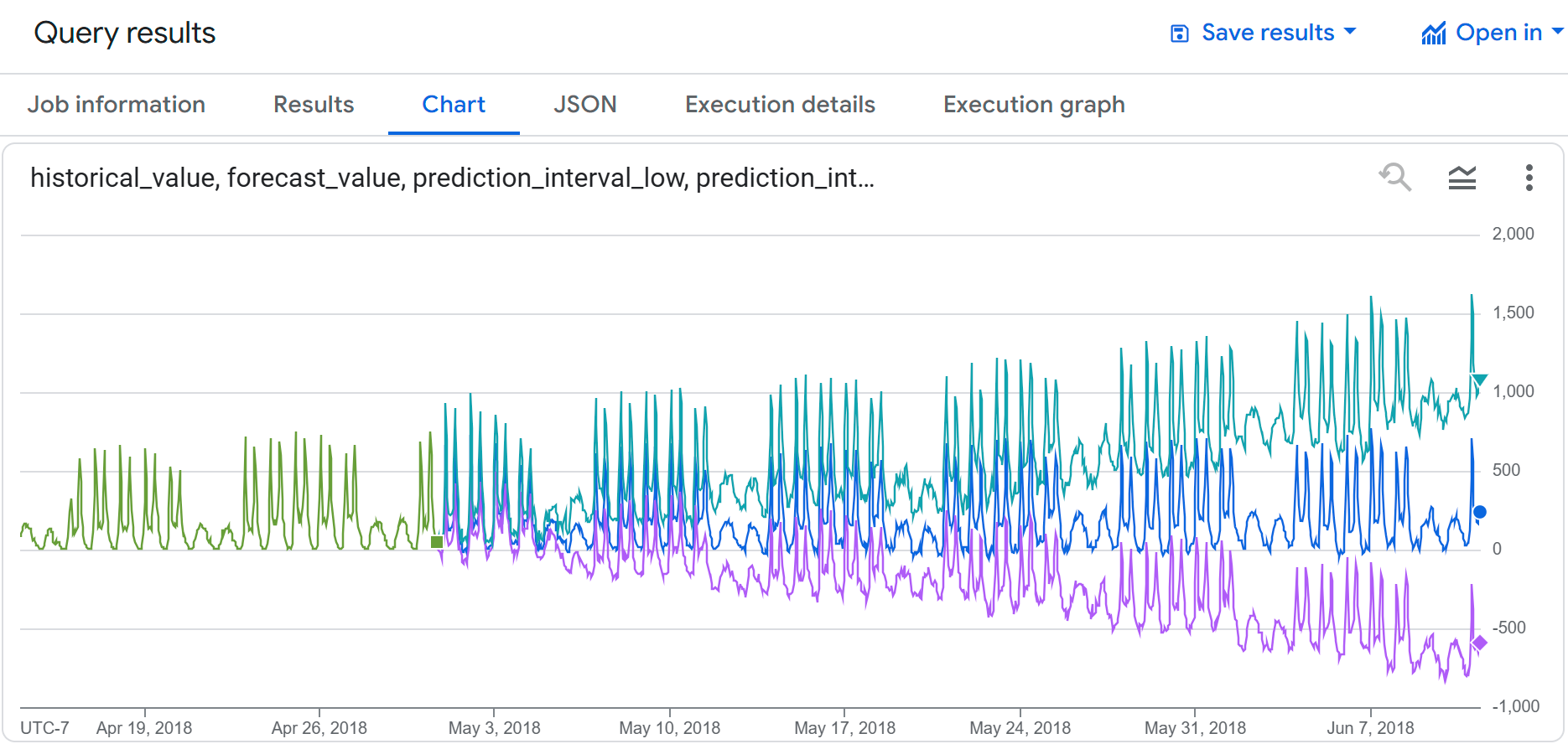
Puedes ver que los datos de entrada y los datos previstos muestran un uso similar del uso compartido de bicicletas. También puedes ver que los límites inferior y superior del intervalo de predicción aumentan a medida que los puntos temporales previstos se alejan más en el futuro.
Previsión de varias series temporales de viajes en bicicleta compartida
La siguiente consulta prevé la cantidad de viajes en bicicleta compartida por tipo de suscriptor y por hora para el próximo mes (aproximadamente 720 horas), según los datos históricos de los últimos cuatro meses. El argumento confidence_level indica que la consulta genera un intervalo de predicción con un nivel de confianza del 95%.
Sigue estos pasos para prever datos con el modelo TimesFM:
En la consola de Cloud de Confiance , ve a la página BigQuery.
En el editor de consultas, pega la siguiente consulta y haz clic en Ejecutar:
SELECT *
FROM
  AI.FORECAST(
    (
      SELECT TIMESTAMP_TRUNC(start_date, HOUR) as trip_hour, subscriber_type, COUNT(*) as num_trips
      FROM `bigquery-public-data.san_francisco_bikeshare.bikeshare_trips`
      WHERE start_date >= TIMESTAMP('2018-01-01')
      GROUP BY TIMESTAMP_TRUNC(start_date, HOUR), subscriber_type
    ),
    horizon => 720,
    confidence_level => 0.95,
    timestamp_col => 'trip_hour',
    data_col => 'num_trips',
    id_cols => ['subscriber_type']);
Los resultados son similares a los siguientes:
+---------------------+--------------------------+------------------+------------------+---------------------------------+---------------------------------+--------------------+
| subscriber_type     | forecast_timestamp       | forecast_value   | confidence_level | prediction_interval_lower_bound | prediction_interval_upper_bound | ai_forecast_status |
+---------------------+--------------------------+------------------+------------------+---------------------------------+---------------------------------+--------------------+
| Subscriber          | 2018-05-01 00:00:00 UTC  | 26.3045959...    |            0.95  | 21.7088378...                   | 30.9003540...                   |                    |
+---------------------+--------------------------+------------------+------------------+---------------------------------+---------------------------------+--------------------+
| Subscriber          |  2018-05-01 01:00:00 UTC | 34.0890502...    |            0.95  | 2.47682913...                   | 65.7012714...                   |                    |
+---------------------+-------------------+------------------+-------------------------+---------------------------------+---------------------------------+--------------------+
| Subscriber          |  2018-05-01 02:00:00 UTC | 24.2154693...    |            0.95  | 2.87621605...                   | 45.5547226...                   |                    |
+---------------------+--------------------------+------------------+------------------+---------------------------------+---------------------------------+--------------------+
| ...                 | ...                      |  ...             | ...              | ...                             |  ...                            |                    |
+---------------------+--------------------------+------------------+------------------+---------------------------------+---------------------------------+--------------------+
Realiza una limpieza
Para evitar que se apliquen cargos a tu cuenta de Google Cloud por los recursos usados en este instructivo, borra el proyecto que contiene los recursos o conserva el proyecto y borra los recursos individuales.
Borra tu proyecto
Para borrar el proyecto, haz lo siguiente:
- En la Cloud de Confiance consola, ve a la página Administrar recursos.
- En la lista de proyectos, elige el proyecto que quieres borrar y haz clic en Borrar.
- En el diálogo, escribe el ID del proyecto y, luego, haz clic en Cerrar para borrar el proyecto.
¿Qué sigue?
- Para obtener una descripción general de BigQuery ML, consulta Introducción a la IA y el aprendizaje automático en BigQuery.